Spectral Signatures Clustering

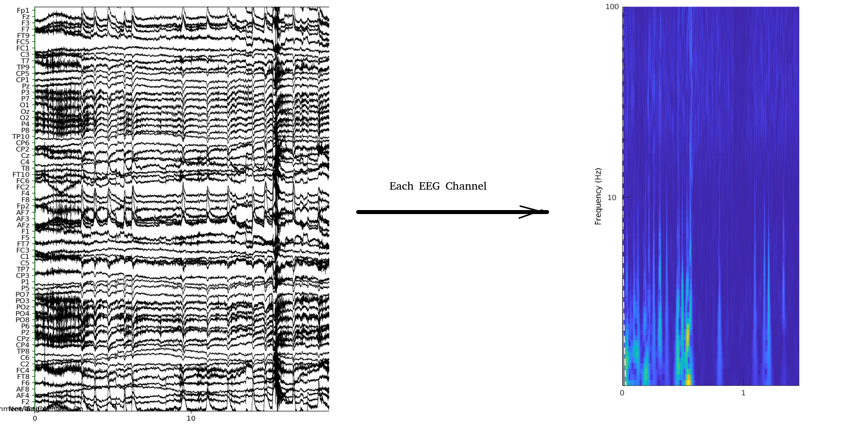
To analyse the continuous EEG data, and to compare their contents in between experimental conditions and channels, we have devised an analysis pipeline which can be summarised as follows. In this study, we recorded the EEG signals using a 64-channel recording system. Each channel records a time-series similar to what we can see in Figure 0.1(a):

Figure 0.1: Each channel time-series is transformed into frequency domain.

We then apply Wavelet transformation to the time-series in each EEG time-series to obtain the variations in the frequency content. To do so, we use the Morse Wavelet transform with time bins of 100 ms as implemented in the cwt function in Matlab. We limit the output frequency to the [1 Hz, 100 Hz] (The EEG signals are recorded with a sampling frequency of 500 Hz). The frequency values for each bin are automatically calculated by the cwt function based on 10 âĂÝvoices per octaveâĂŹ. With these parameters, the resulting matrix will have Nf = 67 rows and the numbers of columns will depend on the length of the EEG time series.

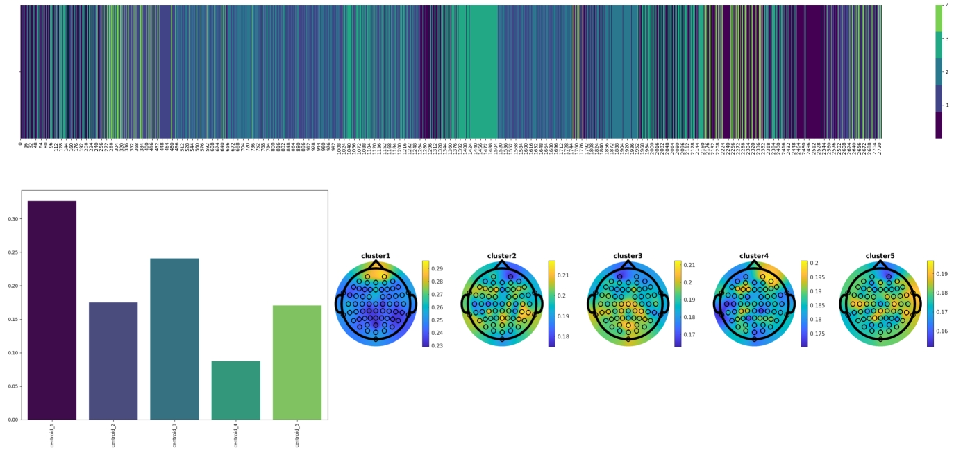
This means that for this experiment, we end up with millions of such matrices, and we should use the proper methodology to distinguish variations specific to each experimental condition. We first bundle the frequency content in each time-bin to frequency or frequencies of interest. For example, if we are only interested in the alpha range, i.e. [8-12Hz] range, we average the values corresponding to all frequencies that fall into this range, and we obtain a scalar value for each time-bin. If we want to consider all conventional frequency ranges, i.e. theta [4-8 Hz], alpha [8-12 Hz], beta [12-20 Hz], low-gamma [20-50 Hz] and high-gamma [50-100 Hz], and run the analysis on all these ranges simultaneously, we average over each range and then replace the original array of size Nf with an array of size 5 (one scalar value for each frequency range). In the next step, we apply a clustering algorithm (in this case, K-means clustering) over all these scalar or array of values for all channels, subjects and stimuli. The choice of the number of clusters can be specified using standard methods such as elbow-test combined with trial and error. Figure a3 shows the centroids when we bundle frequencies into five conventional ranges. Each row is a centroid.

Figure 0.2: The top plot shows the frequency domain data, but now each bin is replaced with the cluster number to which it belongs. Bottom left shows the distribution of each of the five clusters in the data segment, or what I call the spectral signature of the data. Bottom right shows the same data, for all the EEG channels, using a topographical map.

Now we can replace the original values of each bin with its cluster number (in this example, integers in 1-10 range). This means that the matrix of size Nf x Nb [Nb is the number of bins in the EEG time series] is replaced by an array of size 1 x Nb of integer values, each representing a cluster, as shown in 0.2(a).

Now, counting the number/percentages of each cluster in the signal of interest can give us the distribution of clusters in each segment of the EEG signals, which is what we call the Spectral Signature of each EEG signal. The Figure 0.2(b) shows the spectral signature of an EEG time series for an electrode under a given experimental condition and for one participant.

Comparing the spectral signatures between different experimental conditions, channels and subjects can clearly show us what are the variations in the spectral content for each one. When we repeat this process for each channel of each recording, an combining them into a topographical map, we will get a plot such as the one in 0.2(c).