3 Working with PyFDAP

3.1 The PyFDAP main window

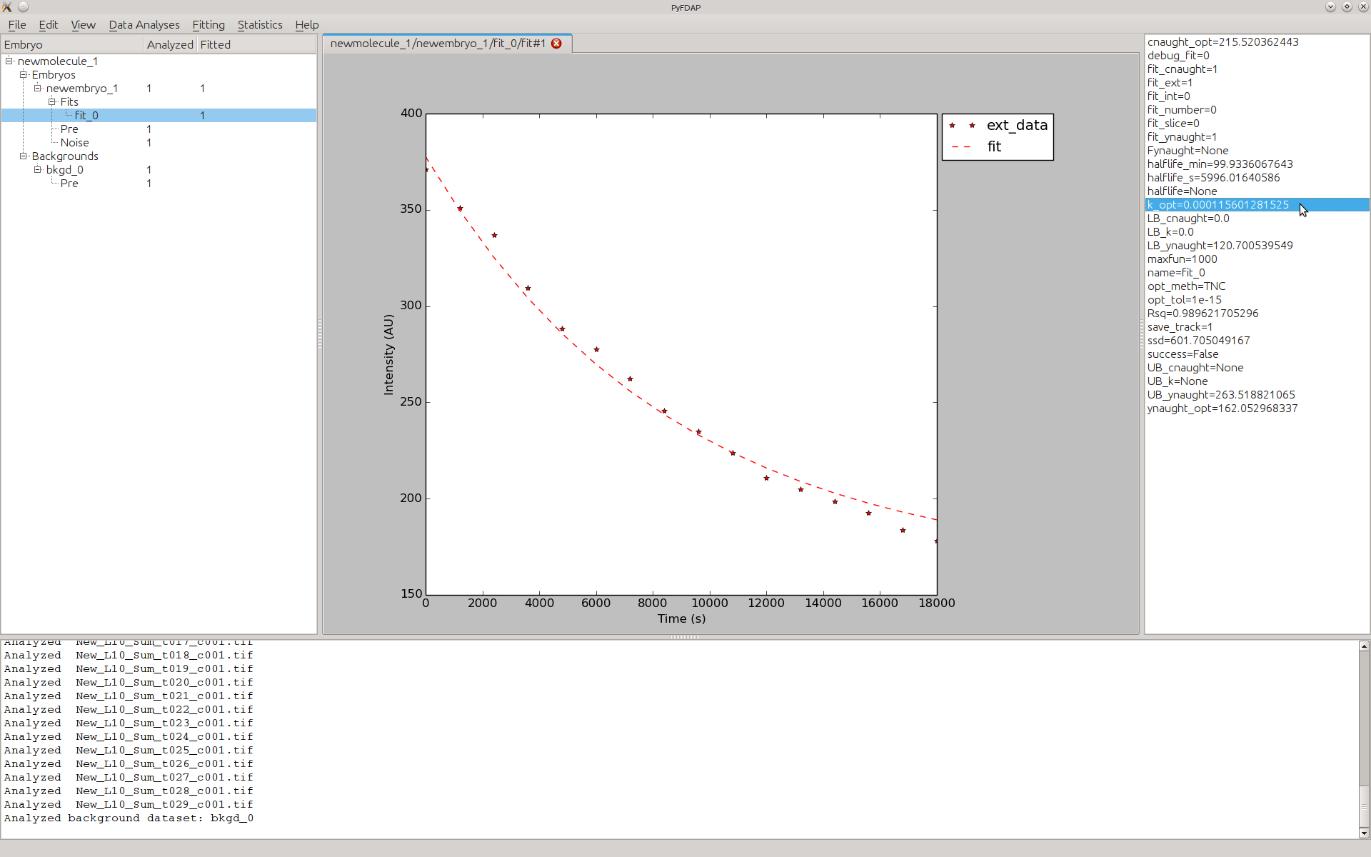
The PyFDAP main window consists of four major compartments: The object list on the left-hand side (red), the property list on the right-hand side (blue), the plot tab in the center (green), and the console at the bottom (magenta).

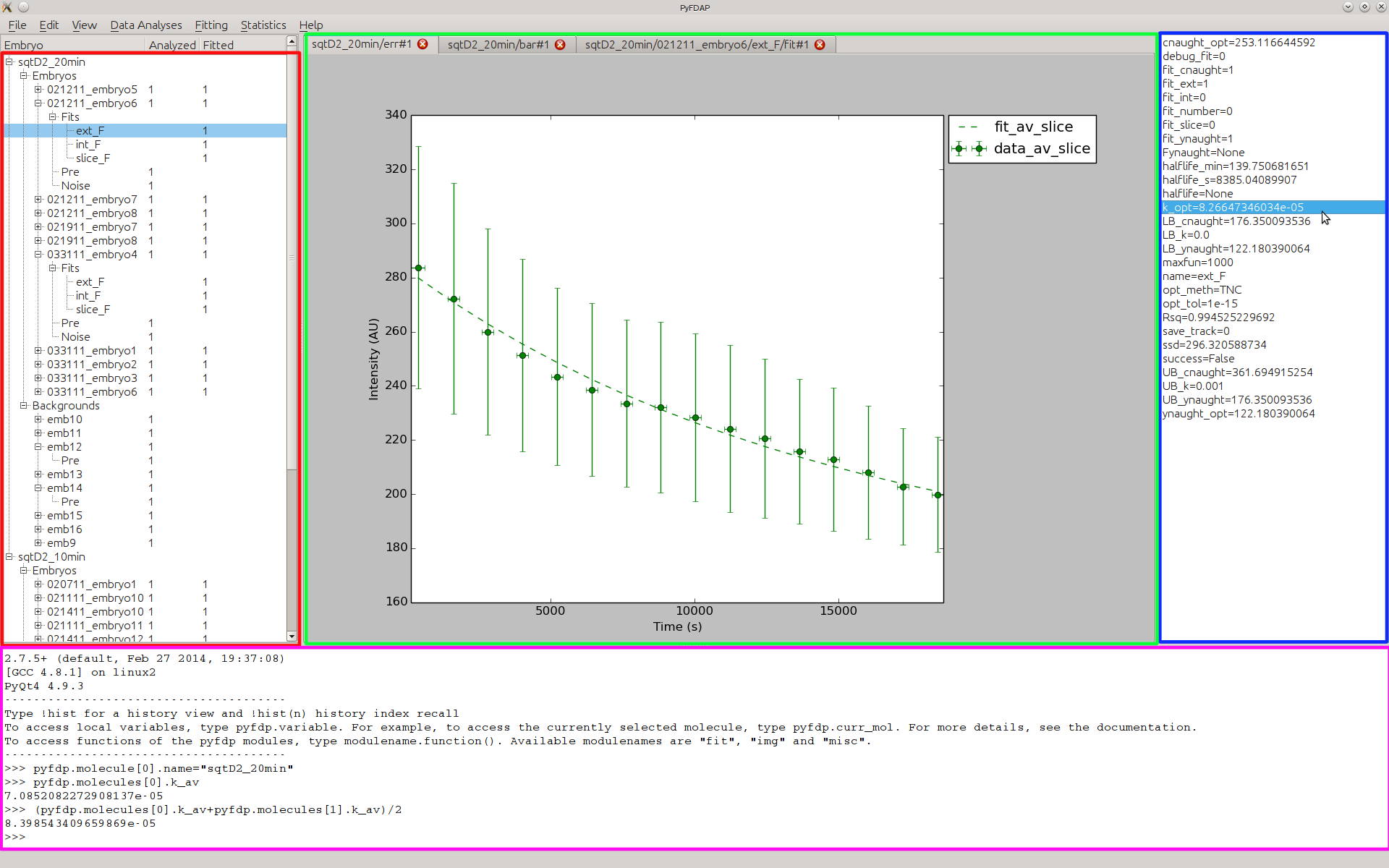
After creating a new molecule, FDAP, background dataset, or fit, the newly created object is shown in the object list according to its hierarchical structure (see Section 4). To inspect the object properties, double-click on the object of choice. The object properties are then listed in the property list on the right-hand side. Many functions in PyFDAP will require you to select the right type of object and will return an error message if not done so.

PyFDAP provides the user with several plotting options. Each plot opens in a new tab with a name according to the currently selected object and the plot type. You can easily switch between plots by clicking on the open tabs.

PyFDAP also comes with an internal Python console. NumPy and the three main PyFDAP modules img, fit, misc are automatically imported. You can use the console to manipulate all PyFDAP objects such as molecules and embryos (FDAP datasets), call other Python functions or simply let PyFDAP return molecule or embryo properties such as longer vectors that are not shown in the property list. PyFDAP also uses the console for debugging outputs, so having a look at the console is often useful.

All major PyFDAP functions can be found in the menu bar at the top of the PyFDAP window. The menus are sorted according to the normal workflow of FDAP experiment analysis.

3.2 First steps with PyFDAP

We provide a fully analyzed FDAP dataset on our website. If you wish to try out PyFDAP using this test dataset, go to http://people.tuebingen.mpg.de/mueller-lab, download the test dataset TestDataset.zip, and unzip it to your PyFDAP folder. If you wish to put it somewhere else, you need to adjust some paths in the molecule file in PyFDAP later. You can now analyze the raw images of the test dataset or your own data (see Section 3.2.1), or you can load a pre-analyzed dataset (see Section 3.2.2).

3.2.1 Analyzing an FDAP dataset

The following section guides you through the major steps of how to use PyFDAP to analyze and fit FDAP datasets if you wish to perform your own FDAP analysis.

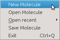
Create a new molecule project by clicking on File → New Molecule.
Change the name of the molecule project by clicking on Edit → Edit Molecule.
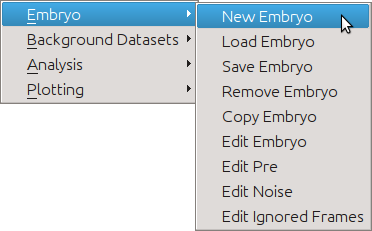
Add a new embryo object (FDAP measurement):
1. Go to Data Analyses → Embryo → New Embryo
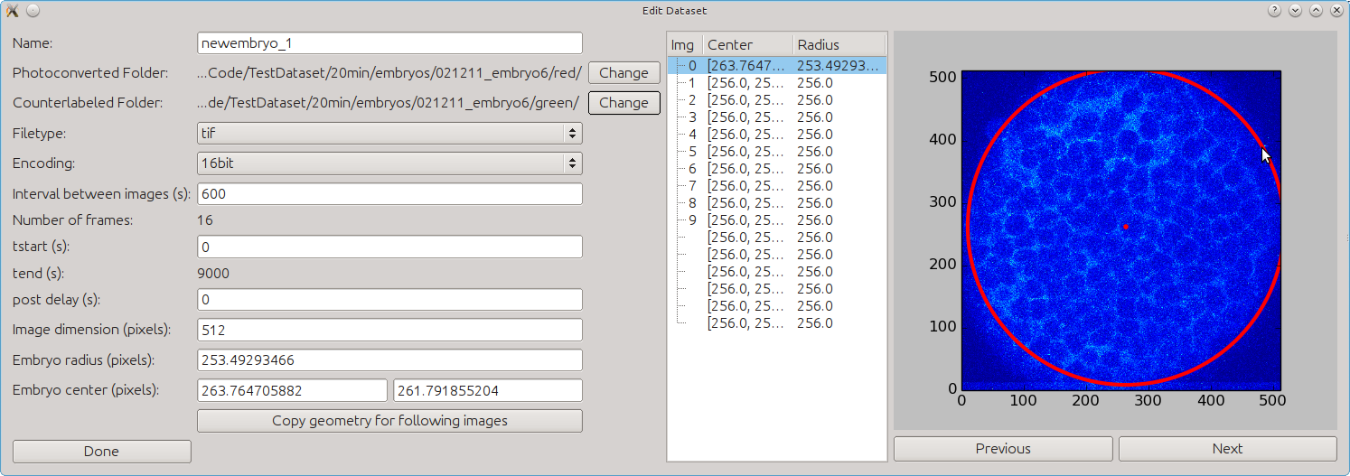
2. Choose the photoconverted folder (images of photoconverted proteins) and counter-labeled folder (images of cell-tracing molecules, e.g. Alexa488-Dextran). For the test dataset, these can be found in the folder TestDataset/squint-dendra2_20min-interval/embryo6/post; the photoconverted folder is called red, and the counter-labeled folder is called green.
3. Enter the dataset-specific properties such as intervals between images (20 min = 1200 s for the test dataset), post-delay (delay between first and second post-conversion pictures resulting from re-adjustment), and center and radius for each image. You can easily select the center and the radius for each image by clicking on the picture. The first click will define the center, the second the radius, and the third click will delete both selections. If you wish to copy the selected radius and center for all following images, click on Copy geometry for following images. When you are done defining the dataset, click on Done.
4. The next pop-up window will allow you to set the “photoconverted” folder, counter-labeled folder, and specific properties of the pre-conversion images similar to the post-conversion dataset in steps (b) and (c). For the test dataset, these can be found in TestDataset/squint-dendra2_20min-interval/embryo6/pre; the “photoconverted” folder is called red, and the counter-labeled folder is called green.
5. The third pop-up window will allow you to define the method of noise calculation. You can choose between three methods:
  - Outside will average intensities outside of the selected radius for each image defined in (c) and then average over all of the calculated averages.
  - Predefined gives you the possibility to enter a value for the noise level yourself.
  - Separate Dataset lets you analyze a separate dataset taken to calculate noise levels. These images are generally taken before or after the experiments without a sample.
  After clicking Done, all important settings for the embryo object are entered.
6. You can add additional embryo objects (FDAP measurements) to the molecule by repeating steps (a) - (e).
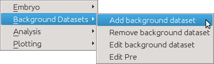
Add a new background object:
1. Go to Data Analyses → Background Datasets → Add background dataset.
2. Choose the “photoconverted” folder (images of “photoconverted” proteins) and counter-labeled folder (images of cell-tracing molecules). For the test dataset, these can be found in TestDataset/squint-background_20min-interval/embryo10/post; the “photoconverted” folder is called red, and the counter-labeled folder is called green.
3. Similar to the embryo object, select parameters specific to the dataset by using the given text fields or by clicking on the image.
4. The next pop-up window will allow you to set the folders and properties of the pre-conversion images of the background dataset similar to the post-conversion dataset. For the test dataset, these can be found in TestDataset/squint-background_20min-interval/embryo10/pre; the “photoconverted” folder is called red, and the counter-labeled folder is called green.
5. After clicking Done, all important settings for the background object are entered. You can add additional background objects to the molecule by repeating steps (a) - (d).
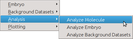
Analyze the molecule project by going to Data Analyses → Analysis → Analyze Molecule. This can take several minutes depending on the amount of datasets added to the molecule project (see Section 5).

The image analysis progress will be printed into the PyFDAP console.
Double-click on the embryo object you want to analyze and add a new fit object:
1. Go to Fitting → Fits → New fit.
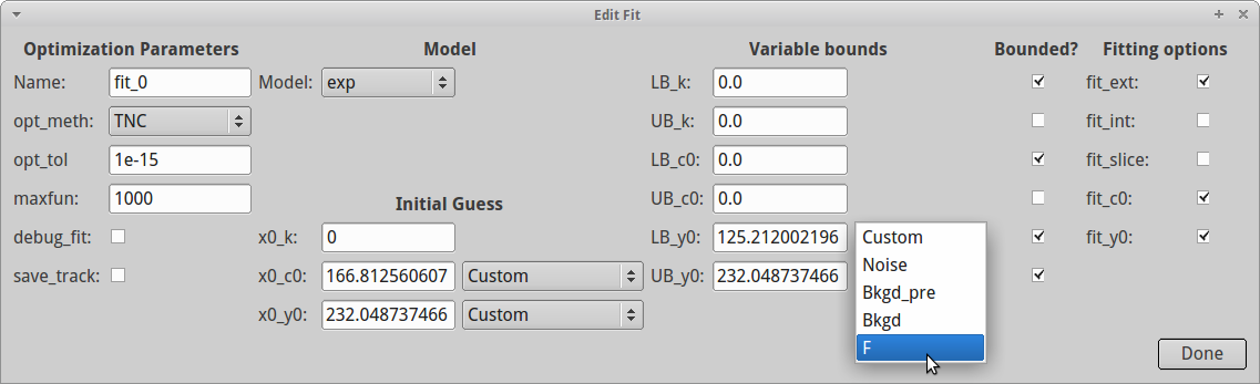
2. Enter the parameters of the fit. The most important are:
  - opt_meth is the optimization method (see Table 3 for details) used for finding the minimum of the SSD (sum of squared differences).
  - opt_tol is the level of tolerance (i.e how good the fit needs to be) given to the optimization algorithm.
  - maxfun is the maximum number of iterations used by the optimizer.
  - Model is the underlying decay model used for the fit. See Section 6.1 for more information.
  - x0_k, x0_c0, x0_y0 are the initial guesses for the three parameters k, c₀, and y₀.
  - LB_k, UB_k, LB_c0, UB_c0, LB_y0, UB_y0 are the lower and upper bounds for the three parameters k, c₀, and y₀ given to the optimizer. You can use the checkboxes to set each variable bounded or unbounded from below and above. For the lower bound of y₀, PyFDAP offers several presets:
    - Custom allows you to enter a value yourself.
    - Noise takes the level of noise as the lower bound for y₀.
    - Bkgd_pre takes the level of the background pre-conversion images as the lower bound for y₀.
    - Bkgd takes the average background level as the lower bound for y₀.
    - F takes the weighting function given in Müller et al. (2012) as the lower bound for y₀.
    More details on the estimation of initial guesses and variable bounds can be found in Section 6.2. Note that not all optimization algorithms offer bounded optimization (see Section 6.3 for more details).
  - fit_ext, fit_int, fit_slice define which regions of the images need to be fitted. You can only select one of the three regions intracelluar, extracelluar, and slice (i.e. total imaged domain) to be fitted during one particular fit.
  - fit_c0, fit_y0 are flags on which parameters are kept fixed and which are free. If a parameter is unchecked, the optimization algorithm will keep this parameter at its initial guess value.
  - After clicking Done, all important settings for the fit object are entered. The fit is performed instantly, and you will see the fitted data. To inspect the optimal parameters resulting from the fit, double-click on the current fit and look in the property list on the right-hand side for k_opt (the decay rate constant) and halflife_min (the half-life in minutes).
3. You can add additional fit objects to the molecule project by repeating steps (a) and (b) described above.
If you changed any settings of a fit (by selecting Fitting → Fits → Edit fit) and want it to be performed again, select the fit in the left column and go to Fitting → Perform Fits → Perform fit.
If you have added and fitted multiple embryo objects (FDAP measurements) and wish to find the average fit over all embryo objects, go to Statistics → Plotting → Plot average fit (see Section 3.3 for details).

3.2.2 Loading a pre-analyzed dataset

Launch PyFDAP, go to File → Open Molecule, and select the file TestDataset/results/TestDataset_20min.pk. You have now successfully loaded a molecule project including one embryo object (FDAP dataset) and one background dataset. You can now try out all features of PyFDAP including all plotting functions.

3.3 Making use of statistical functions in PyFDAP

PyFDAP comes with a few statistical tools for data averaging and analysis. To average the fits from multiple embryo objects (FDAP measurements), go to Statistics → Average Molecule. A pop-up window will ask you to select fits from different embryo objects:

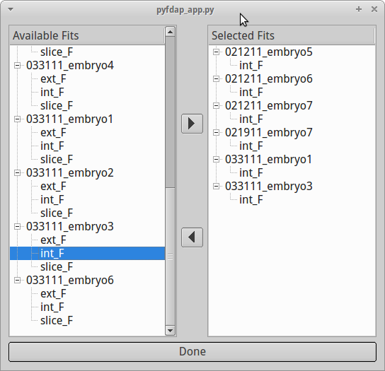
You can add the fits that you want to be considered for averaging to the selection on the right-hand side by double-clicking on the particular fit or by using the arrow buttons on the screen. You can also remove fits from the selection by double-clicking or by using the arrow buttons. Note that for averaging to work, you can only select fits of the same region, e.g. you cannot average a fit for the extracellular region with one for the intracellular region. It is also not possible to let two fits of the same embryo object contribute to the averaged fit.

After selecting the fits that you want to include for averaging, press Done. PyFDAP will automatically compute averages of all important fitting parameters and display them in the property list on the right-hand side. Details on how these averages are computed can be found in Section 6.4. After averaging a selection of fits, you can use PyFDAP’s bar plot functions to compare fitting results from different embryos. Go to Statistics → Plotting and choose between Plot ks by fit, Plot y0s by fit, Plot c0s by fit to plot each of the parameters by fit in a bar plot, or choose Plot all parameters by fit to plot all three optimal parameters by fit.

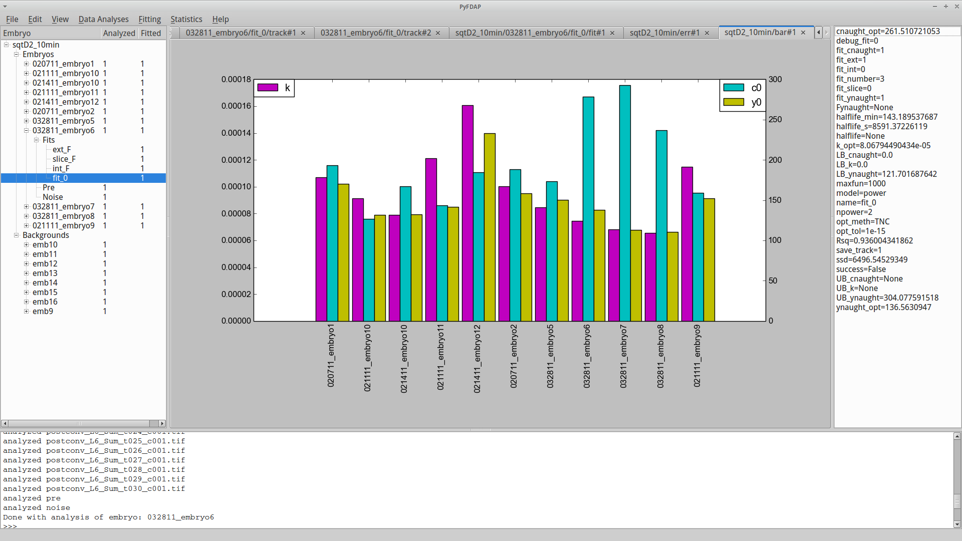
This plot allows you to identify fits that produce parameters strongly deviating from the mean. You can then go back to those fits and adjust the fitting parameters to optimize your final result.

You can also plot the averaged time-dependent fluorescence decay data as error bar plots for unnormalized data or for data normalized between values of 0 and 1. To generate these plots, go to Statistics → Plotting → Plot average fit or Statistics → Plotting → Plot normed average fit.

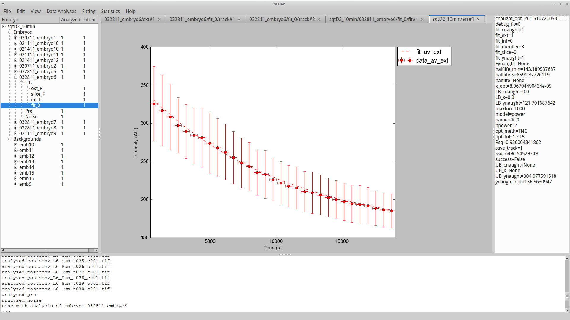
Mathematical details for error bar computation and data normalization can be found in Section 6.4.

3.4 Saving results from PyFDAP

PyFDAP offers multiple ways to save and share FDAP project data and details such as plots, videos, analysis settings, and whole molecule projects.

3.4.1 Saving figures and movies

In Data Analysis → Plotting, users can find plotting commands for

Data and background images for the whole region (slice) as well as for extra- and intracellular domains
Masked images for the whole region (slice) as well as for extra- and intracellular domains
Masks for the whole region (slice) as well as for extra- and intracellular domains
Analysis results for all three regions including background values

Moreover, users can plot fitting results and the fitting progress under Fitting → Plotting. Single plot frames can be saved as *.png, *.pdf, *.eps, *.jpg, *.pgf, *.ps, *.rgba, *.svg, or *.tif. In order to edit the plots using a vector graphics software, we recommend saving images as *.pdf or *.eps files.

PyFDAP also allows users to export image series (such as the fitting progress) as *.mpg or *.avi movies for presentation purposes. Note that PyFDAP does not automatically provide the necessary package for the conversion of image files to movie files; more information about the installation process to enable video output can be found in Section 2.3.

3.4.2 Saving molecule and embryo files

Users can save their molecule sessions to JavaScript Object Notation (JSON) object files. These object files follow the logical hierarchical structure explained in Section 4 and contain all of the data used for the FDAP analysis as well as the fitting results. The molecule and embryo files can be re-loaded into PyFDAP to enable researchers to continue working on a session and to facilitate collaboration among researchers in different locations.

3.4.3 Saving plots and results as .csv files

Plots as well as molecule and embryo objects can also be saved as comma-separated value files that can then be read into other plotting or analysis software such as Excel or Matlab. The molecule and embryo *.csv files follow the hierarchical system of the JSON files (see above). Note that image data will not be exported to *.csv files.