6 Mathematical background
6.1 Decay models
PyFDAP supports two different decay models: Linear- and non-linear decay. Linear decay is given by the ordinary differential equation (ODE)
 |
where c is the concentration of a molecule and k is the rate constant of the decay. Since we assume that the level of fluorescence is proportional to the molecule concentration, we can substitute the concentration with fluorescence intensity. Solving this ODE results in
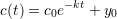 |
where c(t) is the concentration of a molecule at time t, c(0) = c0 is the concentration at time t = 0, and y0 is the baseline fluorescence intensity to which the population of decaying molecules converges. In terms of fluorescence intensity, y0 resembles the baseline level of noise and autofluorescence. From k we can then compute the molecule’s half-life τ by
 |
Some molecules are proposed to decay non-linearly (Eldar et al., 2003), and we have
 |
where n > 1 is the degree of non-linearity and k is the decay rate constant of the molecule. We can solve this ODE and obtain the power-law solution
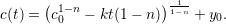 |
For the case of a non-linear decay model, we compute the molecule’s half-life by
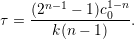 |
6.2 Estimation of initial guesses and bounds for variables
PyFDAP offers multiple options to calculate initial guesses and bounds for variables that are used by
the fitting algorithms to obtain biologically reasonable estimates based on noise, pre-conversion, and
background measurements (see Section 4).
Initial guess for the estimation of c0: A good estimate for c0 is the difference between the pre-conversion and the first post-conversion image, i.e.
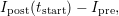 |
where Ipost and Ipre are the fluorescence intensities after and before photoconversion, respectively,
and tstart is the time at which the first image was taken.
Initial guess for the estimation of the baseline y0: PyFDAP offers the two presets Ipost(tstart) and
Ipost(tend), where tend is the time at which the last image was taken and where protein decay should
be almost complete. Our tests showed that the optimization algorithms worked well if y0,opt is
approached from above using Ipost(tstart) as the initial guess for y0.
Estimation of the lower bound for the baseline y0: This estimate is a crucial part of the fitting process. PyFDAP offers several algorithms to perform this estimation based on the amount and quality of the data available.
- The simplest estimate of the lower bound of y0 is the average background noise of the measurements . Due to autofluorescence of the samples, this estimate is generally too low, but it serves as the lower bound of the lower bounds of y0.
- Alternatively, the lower bound of the baseline y0 can be estimated from the average level
of autofluorescence represented by
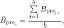
where r ∈{intracellular, extracellular, entiredomain} is the investigated region, and j ∈{1,...,b} are the indices of background pre-conversion datasets with intensities Bprej,r.
- PyFDAP also offers the possibility to use the average background intensity as the lower bound
of the baseline y0:

where j,r is the mean intensity in region r of a background dataset over all data points given by
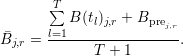
Here, tl with l ∈{1,...,T} is the time when the l-th image was taken and T is the number of post-conversion images.
- PyFDAP includes a special weighting function F (Müller et al., 2012) given by
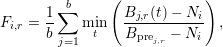
where i is the current FDAP measurement, r is the investigated region, and j is the index of background datasets with intensities B(t) at time t. Here, the noise measurement of measurement i is given by Ni. Using the function F, users can compute the lower bound of the baseline y0i,r for measurement i and region r by

where Iprei,r denotes the pre-conversion intensity of the FDAP measurement i in region r.
6.3 Optimization algorithms
PyFDAP comes with a wide selection of optimization algorithms taken from the SciPy optimize package (http://docs.scipy.org/doc/scipy/reference/optimize.html) (Nelder and Mead (1965); Polak and Ribière (1969); Broyden (1970); Goldfarb (1970); Fletcher (1970); Shanno (1970); Nash (1984); Kraft (1988); Byrd et al. (1995); Nocedal and Wright (2006)). A list of all optimization algorithms available in PyFDAP can be found in Table 3.
Method | Name in PyFDAP | Type | Reference |
Limited-memory BFGS | L-BFGS-B | quasi-Newton | |
Truncated Newton Conjugate | TNC | Newton conjugate | |
Sequential Least Squares Programming | SLSQP | sequential quadratic | |
Brute force | brute | brute force | SciPy Reference Guide |
Nelder-Mead | Nelder-Mead | simplex | |
Broyden-Fletcher-Goldfarb-Shanno | BFGS | quasi-Newton |
Broyden (1970); Goldfarb (1970); Fletcher (1970); Shanno (1970) |
Nonlinear Conjugate Gradient | CG | Newton conjugate | |
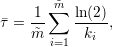
6.4 Statistics
PyFDAP can average over multiple fits from different embryo objects (FDAP measurements). Details of how to select fits for averaging are described in Section 3.3.
PyFDAP averages the optimal parameters for k, y0, c0, and protein half-lives τ through an arithmetic mean. For example, the average decay rate constant is obtained by
 |
where  is the number of fits to be averaged. The average half-life can be computed in two ways
resulting in different average half-lives. PyFDAP computes the average half-life through the
arithmetic mean given by
is the number of fits to be averaged. The average half-life can be computed in two ways
resulting in different average half-lives. PyFDAP computes the average half-life through the
arithmetic mean given by
 |
For the linear decay model, this yields
 | (1) |
and in the case of the non-linear decay model we obtain
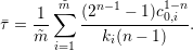 | (2) |
However, computing the average half-life directly from the average decay rate yields
 | (3) |
for the linear decay model and
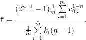 | (4) |
in case of the non-linear decay model. It is obvious that equations 1 and 3 as well as equations 2 and 4 do not produce the same half-lives, and the user needs to decide which way of half-life computation is appropriate for the application.
PyFDAP can produce different error bar plots for each averaged region. Clicking on Statistics → Plotting → Plot average fit will result in a plot in which each average data point (tj) is computed as the arithmetic mean
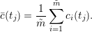 |
Error bars are computed as the standard deviation for each time tj. Clicking on Statistics → Plotting → Plot normed average fit returns a plot in which all data points are normalized between values of 0 and 1. The normalization is performed by subtracting the baseline value y0,i from each data point and dividing the result by c0,i, i.e.
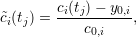 |
where  (tj) is the normalized data point at time tj. This normalization facilitates the comparison of
decay curve shapes, but it substantially changes the meaning of the error bars. Since all
data series are pinned to a value of 1 at their first time point, the standard deviation
vanishes for this data point. The following data points will generally produce increasing
error bars since the decay curves generally diverge. The length of the normalized error
bars can be interpreted as the extent to which the decay curves diverge throughout the
experiments.
(tj) is the normalized data point at time tj. This normalization facilitates the comparison of
decay curve shapes, but it substantially changes the meaning of the error bars. Since all
data series are pinned to a value of 1 at their first time point, the standard deviation
vanishes for this data point. The following data points will generally produce increasing
error bars since the decay curves generally diverge. The length of the normalized error
bars can be interpreted as the extent to which the decay curves diverge throughout the
experiments.